Analysing records¶

This page outlines methods of analysis of process metrics recordings produced with procpath record.

Visualisation¶

Graphical visualisation is the most straightforward way to interpret time series data.

Built-in¶

Procpath comes with built-in SVG visualisation for temporal process analysis. The data for visualisation can be fetch from the SQLite database in 3 ways:

Built-in named queries, which can be used like --query-name rss or --query-name cpu.

Note that some named queries require recording of procfiles (i.e. what’s passed to --procfile-list) that are not enabled by default. Here’s the list of all registered named queries with their requirements:
```
- cpu: []
- rss: []
- pss: ['smaps_rollup']
- uss: ['smaps_rollup']
- swap: ['smaps_rollup']
- fd: ['fd']
- rbs: ['io']
- wbs: ['io']
- wait: []
```
Custom value SELECT expression for any numeric column, e.g. --custom-value-expr "stat_majflt / 1000.0" with scaling, or --custom-value-expr IFNULL(io_rchar - LAG(io_rchar) OVER (PARTITION BY stat_pid ORDER BY record_id), 0) converting cumulative series to series of deltas.
Custom SQL file with whatever calculation you can think of. The result-set must have 3 columns: ts, pid, value. The built-in queries can be used as an example, see procpath.procret module.

Plotting features include the following (see the listing of plot command).

filtering by time range and PIDs
post-processing using moving average and Ramer-Douglas-Peucker algorithm
comparison plot with two Y axes
logarithmic scale plot
Pygal [1] plot styles and value formatters, and custom plot title

This example plots all processes’ RSS from the recorded database, with moving average window of 4.

procpath plot -d out.sqlite -f rss.svg -q rss -w 4

If opened in a browser alone (e.g. right click the example below and Open Image in New Tab) this SVG has a number interactive features:

legend hover highlights the line
legend click toggles the line
legend double click hides/shows all other lines
X time label hover draws a guideline to indicate intersections
dot hover displays the series name, time and value

This example plots RSS vs CPU for PIDs 10543 and 22570 between 2020-07-26 21:30:00 and 2020-07-26 22:30:00 UTC from the recorded database, with moving average window of 4 and using Ramer-Douglas-Peucker algorithm to remove redundant points from the SVG with ε=0.1, on logarithmic scale and using Pygal’s LightColorizedStyle, forced integer value formatter and without hover dots.

procpath plot -d out.sqlite -q rss -q cpu -p 10543,22570 -l -w 4 -e 0.1 \
  --after 2020-07-26T21:30:00 --before 2020-07-26T22:30:00 \
  --formatter integer --style LightColorizedStyle --no-dots

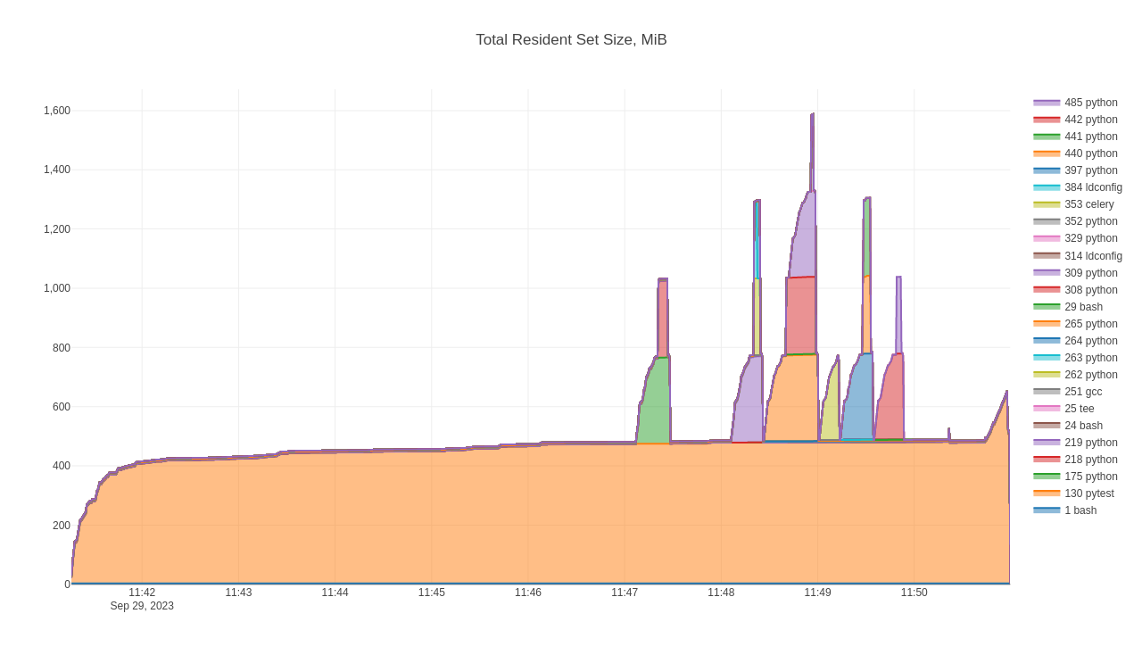
There are a few advanced visualisations that are available only in Sqliteviz via procpath explore (described below). Here follow examples of these visualisation based on a recording of a Pytest run in a GitLab pipeline:

Total Resident Set Size, MiB – shows total RSS and each process’ contribution to it
Process Timeline – shows lifetime off each process; point hover text shows cmdline and path to root process (usually PID 1)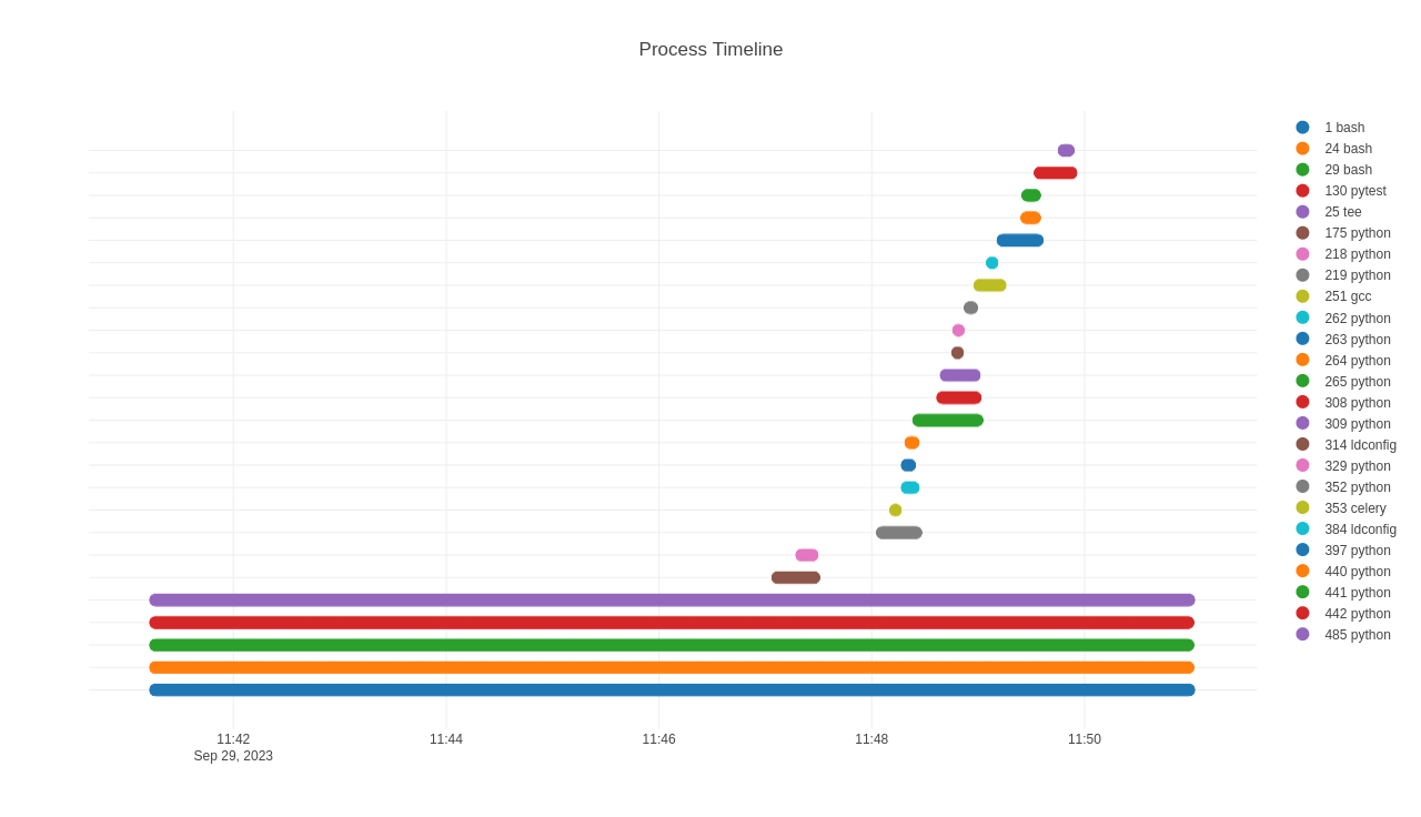
Process Tree – shows parent (stat_ppid) child (stat_pid) process relationship; edge hover text shows cmdline of the child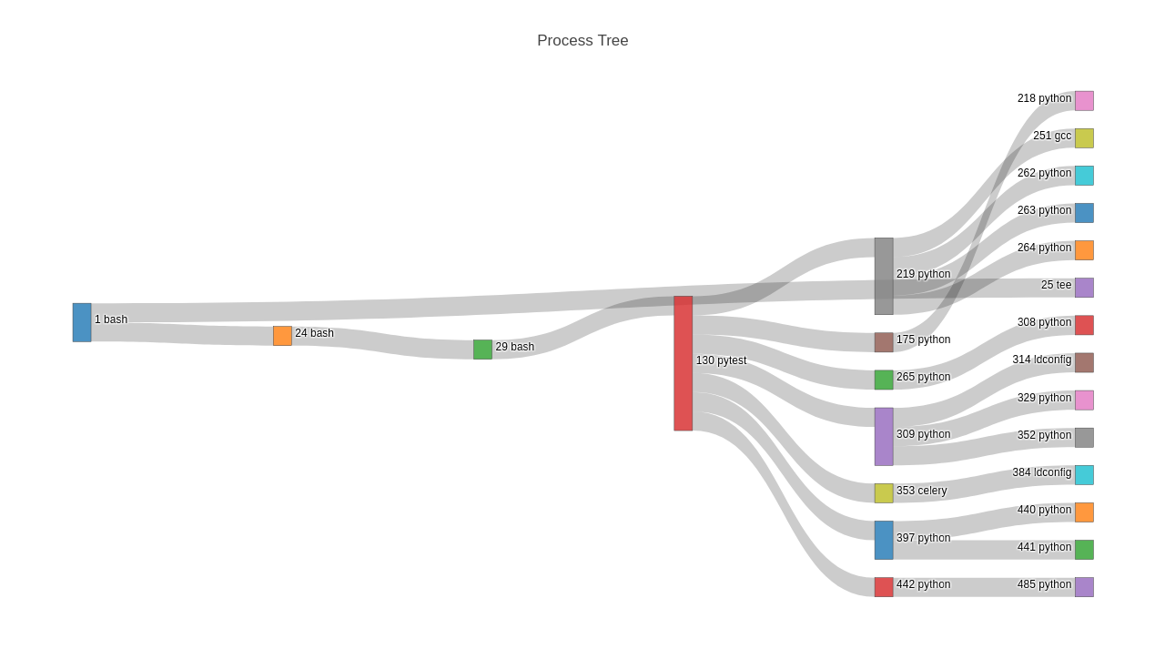

Ad-hoc¶

A GUI-driven ad-hoc visualisation can be done in Sqliteviz [2].

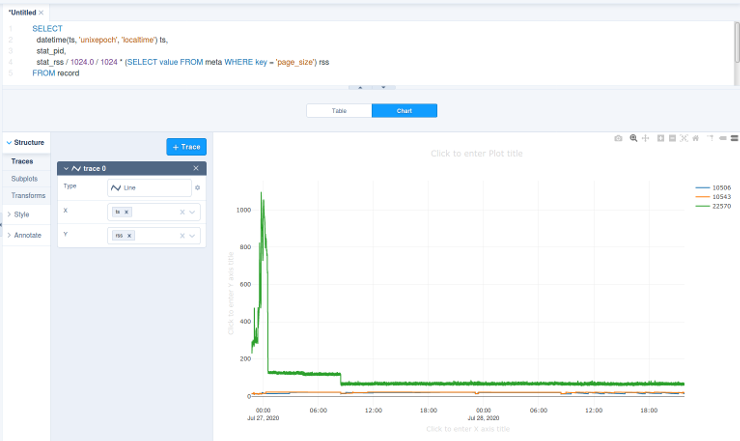
Ad-hoc visualisation in the online version of Sqliteviz is straightforward.

Drop an SQLite database file into Sqliteviz
Create new query
Enter the SQL query (see examples below) and run it
Switch to Chart tab
Click + Trace, select Line chart
Choose X = ts
Choose the expression to plot on Y, for instance, rss
Switch to Transforms, click + Transform, add Split and choose stat_pid

It should look something like this.

Procpath integrates with Sqliteviz via procpath explore. On first execution the command downloads latest GitHub build of Sqliteviz into ~/.cache/procpath, makes Procpath queries (and visualisation for them; also Sqliteviz-only visualisations) available to Sqliteviz, starts an HTTP server from that directory and opens / in the default browser. Subsequent runs use the downloaded version and are fully offline. For the CLI options of the command, see the listing of explore command.

Real-time¶

For live diagnostic of software, having real-time plots of the processes’ metrics may come in handy. Even though procpath record writes every snapshot into the database, which makes it possible to frequently plot it with running procpath plot, possibly limiting the view to the last interval, say the last 1 hour, with --after, it’s still far from real-time.

feedgnuplot [7] (available on Debian family out of official repositories) can used to produce real-time charts fed from the SQLite database being procpath record’ed. A simple Bash sleep-loop iterating sqlite3 with a tail-like query can be used to produce a live chart updating at 1 Hz and showing the last minute worth of data.

while sleep 1; do \
    sqlite3 -separator ' ' 'file:target.sqlite?mode=ro&nolock=1' \
    < tail.sql; \
done \
    | feedgnuplot --stream --domain --dataid --lines --points --xlen 60 \
    --autolegend --set "key outside" \
    --timefmt "%Y-%m-%dT%H:%M:%S" --set "format x '%H:%M:%S'" \
    --title "CPU Usage, %"

Note

Because it’s undesired to interfere with the writing process, the above opens the SQLite database in read-only mode, where SQLite doesn’t expect the database to change. Occasionally, the read coincides with the write and you get this error in the terminal: Error: database disk image is malformed.

It is negligible. Its only effect is the loss of a data-point on the live chart.

The record database can become big, and the query should run under 1 second, the following is an optimised tail query for CPU usage:

WITH RECURSIVE last_snapshot(record_id, ts) AS (
    SELECT *
    FROM (
        SELECT record_id, ts FROM record ORDER BY record_id DESC LIMIT 1
    )
    UNION
    SELECT r.record_id, r.ts
    FROM record r
    JOIN last_snapshot l ON r.record_id = l.record_id - 1 AND r.ts = l.ts
), penultimate_snapshot(record_id, ts) AS (
    SELECT record_id, ts
    FROM record
    WHERE record_id = (SELECT MIN(record_id) - 1 FROM last_snapshot)
    UNION
    SELECT r.record_id, r.ts
    FROM record r
    JOIN penultimate_snapshot p ON r.record_id = p.record_id - 1 AND r.ts = p.ts
), last_two_snapshot_range AS (
    SELECT MIN(record_id) min_id, MAX(record_id) max_id
    FROM (
        SELECT record_id FROM penultimate_snapshot
        UNION
        SELECT record_id FROM last_snapshot
    )
), diff_all AS (
    SELECT
        ts,
        record_id,
        stat_pid,
        stat_utime + stat_stime - LAG(stat_utime + stat_stime) OVER (
            PARTITION BY stat_pid ORDER BY record_id
        ) tick_diff,
        ts - LAG(ts) OVER (
            PARTITION BY stat_pid ORDER BY record_id
        ) ts_diff
    FROM record
    JOIN last_two_snapshot_range ON record_id BETWEEN min_id AND max_id
), diff AS (
    SELECT * FROM diff_all WHERE tick_diff IS NOT NULL
)
SELECT
    strftime('%Y-%m-%dT%H:%M:%S', ts, 'unixepoch') ts,
    '№' || stat_pid,
    100.0 * tick_diff / (
        SELECT value FROM meta WHERE key = 'clock_ticks'
    ) / ts_diff cpu
FROM diff
ORDER BY stat_pid, record_id

And the following for RSS footprint:

WITH RECURSIVE last_snapshot(record_id, ts, stat_pid, stat_rss) AS (
    SELECT *
    FROM (
        SELECT record_id, ts, stat_pid, stat_rss
        FROM record
        ORDER BY record_id
        DESC LIMIT 1
    )
    UNION
    SELECT r.record_id, r.ts, r.stat_pid, r.stat_rss
    FROM record r
    JOIN last_snapshot l ON r.record_id = l.record_id - 1 AND r.ts = l.ts
)
SELECT
    strftime('%Y-%m-%dT%H:%M:%S', ts, 'unixepoch') ts,
    '№' || stat_pid,
    stat_rss / 1024.0 / 1024 * (
        SELECT value FROM meta WHERE key = 'page_size'
    ) rss
FROM last_snapshot
ORDER BY stat_pid, record_id

Put the query into tail.sql and run the Bash snippet above. Other metrics can be tail’ed and plotted similarly.

feedgnuplot should pop up a gnuplot window, if you run it from a graphical session. gnuplot also supports ASCII plotting in the terminal – add --terminal dumb for that. gnuplot supports multiple “terminals” [8] (i.e. rendering engines).

SQL¶

Ad-hoc SQL queries are another way of analysis of process metrics records. Their result sets can be consumed directly, or fed to the built-in or external means of visualisation as described above.

Custom queries¶

For example, you may be interested in programs which at least one time consumed more than 10% of main memory of the system,

SELECT DISTINCT stat_comm
FROM record
WHERE 1.0 * stat_rss / (SELECT value FROM meta WHERE key = 'physical_pages') > 0.1

or in a full timeline of processes each of which at least once consumed more that 10% of a CPU core (e.g. to pin down the source of load spikes).

WITH diff AS (
    SELECT
        record_id,
        ts,
        stat_pid,
        stat_comm,
        stat_utime + stat_stime - LAG(stat_utime + stat_stime) OVER (
            PARTITION BY stat_pid
            ORDER BY record_id
        ) tick_diff,
        ts - LAG(ts) OVER (
            PARTITION BY stat_pid
            ORDER BY record_id
        ) ts_diff
    FROM record
), one_time_pid_condition AS (
    SELECT stat_pid
    FROM diff
    WHERE 100.0 * tick_diff / (
        SELECT value FROM meta WHERE key = 'clock_ticks'
    ) / ts_diff > 10
    GROUP BY stat_pid
)
SELECT
    datetime(ts, 'unixepoch', 'localtime') ts,
    stat_pid pid,
    stat_comm,
    100.0 * tick_diff / (
        SELECT value FROM meta WHERE key = 'clock_ticks'
    ) / ts_diff value
FROM diff
JOIN one_time_pid_condition USING(stat_pid)
WHERE tick_diff IS NOT NULL
ORDER BY stat_pid, record_id

Registered queries¶

The following listing contains the queries registered in Procpath, as used by procpath plot (without their WHERE clauses that correspond to time and PID filters).

-- cpu: CPU Usage, %
WITH diff_all AS (
    SELECT
        record_id,
        ts,
        stat_pid,
        stat_utime + stat_stime - LAG(stat_utime + stat_stime) OVER (
            PARTITION BY stat_pid
            ORDER BY record_id
        ) tick_diff,
        ts - LAG(ts) OVER (
            PARTITION BY stat_pid
            ORDER BY record_id
        ) ts_diff
    FROM record
), diff AS (
    SELECT * FROM diff_all WHERE tick_diff IS NOT NULL
)
SELECT
    ts * 1000 ts,
    stat_pid pid,
    100.0 * tick_diff / (SELECT value FROM meta WHERE key = 'clock_ticks') / ts_diff value
FROM diff;

-- rss: Resident Set Size, MiB
SELECT
    ts * 1000 ts,
    stat_pid pid,
    stat_rss / 1024.0 / 1024 * (SELECT value FROM meta WHERE key = 'page_size') value
FROM record;

-- pss: Proportional Set Size, MiB
SELECT
    ts * 1000 ts,
    stat_pid pid,
    smaps_rollup_pss / 1024.0 value
FROM record;

-- uss: Unique Set Size, MiB
SELECT
    ts * 1000 ts,
    stat_pid pid,
    (smaps_rollup_private_clean + smaps_rollup_private_dirty) / 1024.0 value
FROM record;

-- swap: Swap, MiB
SELECT
    ts * 1000 ts,
    stat_pid pid,
    smaps_rollup_swap / 1024.0 value
FROM record;

-- fd: Open File Descriptors
SELECT
    ts * 1000 ts,
    stat_pid pid,
    fd_anon + fd_dir + fd_chr + fd_blk + fd_reg + fd_fifo + fd_lnk + fd_sock value
FROM record;

-- rbs: Disk Read, B/s
WITH diff_all AS (
    SELECT
        record_id,
        ts,
        stat_pid,
        io_read_bytes - LAG(io_read_bytes) OVER (
            PARTITION BY stat_pid
            ORDER BY record_id
        ) byte_diff,
        ts - LAG(ts) OVER (
            PARTITION BY stat_pid
            ORDER BY record_id
        ) ts_diff
    FROM record
), diff AS (
    SELECT * FROM diff_all WHERE byte_diff IS NOT NULL
)
SELECT
    ts * 1000 ts,
    stat_pid pid,
    byte_diff / ts_diff value
FROM diff;

-- wbs: Disk Write, B/s
WITH diff_all AS (
    SELECT
        record_id,
        ts,
        stat_pid,
        io_write_bytes - LAG(io_write_bytes) OVER (
            PARTITION BY stat_pid
            ORDER BY record_id
        ) byte_diff,
        ts - LAG(ts) OVER (
            PARTITION BY stat_pid
            ORDER BY record_id
        ) ts_diff
    FROM record
), diff AS (
    SELECT * FROM diff_all WHERE byte_diff IS NOT NULL
)
SELECT
    ts * 1000 ts,
    stat_pid pid,
    byte_diff / ts_diff value
FROM diff;

-- wait: I/O wait, %
WITH diff_all AS (
    SELECT
        record_id,
        ts,
        stat_pid,
        stat_delayacct_blkio_ticks - LAG(stat_delayacct_blkio_ticks) OVER (
            PARTITION BY stat_pid
            ORDER BY record_id
        ) tick_diff,
        ts - LAG(ts) OVER (
            PARTITION BY stat_pid
            ORDER BY record_id
        ) ts_diff
    FROM record
), diff AS (
    SELECT * FROM diff_all WHERE tick_diff IS NOT NULL
)
SELECT
    ts * 1000 ts,
    stat_pid pid,
    100.0 * tick_diff / (SELECT value FROM meta WHERE key = 'clock_ticks') / ts_diff value
FROM diff;

Note

Window function support was first added to SQLite with release version 3.25.0 (2018-09-15)
The CPU query above only accounts for user and system time

SQLite GUI¶

Suggested desktop SQLite database explorers suitable for inspection, splitting, merging, exporting and crafting custom queries against process metrics databases are the following.

DB Browser for SQLite [5]

It should be available from the OS repository. And there’s PPA [6] with recent builds.
DBeaver [4]

It can be installed from Flathub, Eclipse Marketplace or its separate Eclipse installer.
SQLiteStudio [3]

Because it’s distributes as pre-built application directory, it’s possible to replace its libsqlite3 with a newer one.

Analysing records¶

Visualisation¶

Built-in¶

Ad-hoc¶

Real-time¶

SQL¶

Custom queries¶

Registered queries¶

SQLite GUI¶

Procpath

Navigation

Related Topics